使用支持向量回归器进行时间序列预测
在上一课中,你学习了如何使用ARIMA模型进行时间序列预测。现在你将学习支持向量回归器模型,这是一种用于预测连续数据的回归模型。
课前测验
引言
在本课程中,你将探索一种使用SVM:Support Vector Machine(支持向量机)构建回归模型的特定方法,即SVR:Support Vector Regressor(支持向量回归器)。
时间序列背景下的SVR 1
在理解SVR在时间序列预测中的重要性之前,你需要了解以下一些重要概念:
- 回归(Regression): 一种监督学习技术,用于从一组给定的输入中预测连续值。其思想是在特征空间中拟合一条能包含最多数据点的曲线(或直线)。点击这里了解更多信息。
- 支持向量机(Support Vector Machine, SVM): 一种监督式机器学习模型,用于分类、回归和异常值检测。该模型是特征空间中的一个超平面,在分类任务中充当边界,在回归任务中充当最佳拟合线。在SVM中,通常使用核函数将数据集转换到更高维度的空间,使其更容易被分离。点击这里了解更多关于SVM的信息。
- 支持向量回归器(Support Vector Regressor, SVR): SVM的一种,用于找到能包含最多数据点的最佳拟合线(在SVM中为超平面)。
为什么选择SVR?1
在上一课中,你学习了ARIMA,这是一种非常成功的用于预测时间序列数据的统计线性方法。然而,在许多情况下,时间序列数据具有非线性特征,这是线性模型无法捕捉的。在这种情况下,SVM在回归任务中考虑数据非线性的能力使得SVR在时间序列预测中取得了成功。
练习 - 构建一个SVR模型
数据准备的前几个步骤与上一课ARIMA的步骤相同。
打开本课的 _/working_ 文件夹,找到 _notebook.ipynb_ 文件。2
-
运行 notebook 并导入必要的库:2
-
从
/data/energy.csv文件中加载数据到 Pandas dataframe 并查看:2 -
绘制从2012年1月到2014年12月所有可用的能源数据:2
Pythonenergy.plot(y='load', subplots=True, figsize=(15, 8), fontsize=12) plt.xlabel('timestamp', fontsize=12) plt.ylabel('load', fontsize=12) plt.show()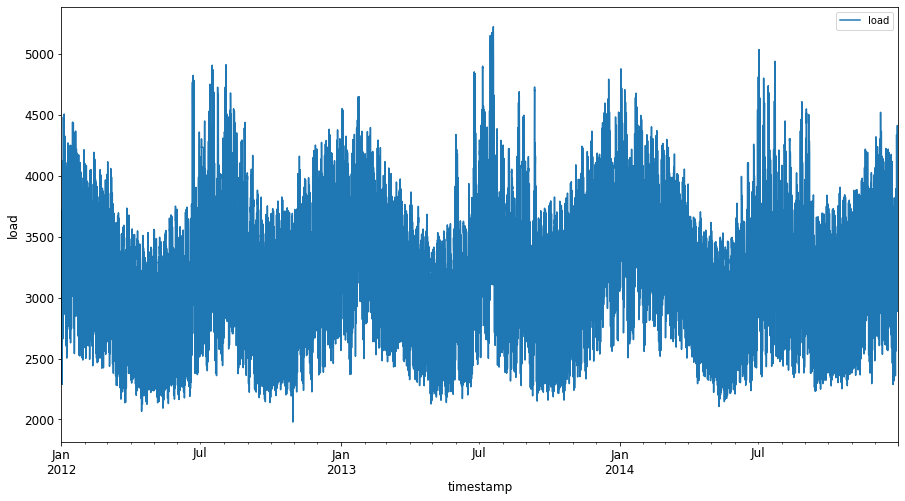
现在,让我们开始构建SVR模型。
创建训练和测试数据集
数据加载后,你可以将其分为训练集和测试集。然后,你将重塑数据以创建一个基于时间步的数据集,这是SVR所需要的。你将在训练集上训练你的模型。模型训练完成后,你将在训练集、测试集和完整数据集上评估其准确性,以观察其整体性能。你需要确保测试集的时间段晚于训练集,以确保模型不会从未来的时间段获取信息2(这种情况称为过拟合)。
-
将2014年9月1日至10月31日这两个月的时间段分配给训练集。测试集将包括2014年11月1日至12月31日这两个月的时间段:2
-
可视化差异:2
Pythonenergy[(energy.index < test_start_dt) & (energy.index >= train_start_dt)][['load']].rename(columns={'load':'train'}) \ .join(energy[test_start_dt:][['load']].rename(columns={'load':'test'}), how='outer') \ .plot(y=['train', 'test'], figsize=(15, 8), fontsize=12) plt.xlabel('timestamp', fontsize=12) plt.ylabel('load', fontsize=12) plt.show()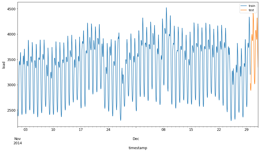
准备用于训练的数据
现在,你需要通过筛选和缩放数据来为训练做准备。筛选你的数据集,只包括所需的时间段和列,并通过缩放确保数据被投射到0到1的区间内。
创建带时间步的数据 1
对于SVR,你需要将输入数据转换为 [批次, 时间步] 的形式。因此,你需要重塑现有的 train_data 和 test_data,增加一个代表时间步的新维度。
在本例中,我们取 timesteps = 5。因此,模型的输入是前4个时间步的数据,输出将是第5个时间步的数据。
使用嵌套列表推导式将训练数据转换为2D张量:
train_data_timesteps=np.array([[j for j in train_data[i:i+timesteps]] for i in range(0,len(train_data)-timesteps+1)])[:,:,0]
train_data_timesteps.shape
将测试数据转换为2D张量:
test_data_timesteps=np.array([[j for j in test_data[i:i+timesteps]] for i in range(0,len(test_data)-timesteps+1)])[:,:,0]
test_data_timesteps.shape
从训练和测试数据中选择输入和输出:
x_train, y_train = train_data_timesteps[:,:timesteps-1],train_data_timesteps[:,[timesteps-1]]
x_test, y_test = test_data_timesteps[:,:timesteps-1],test_data_timesteps[:,[timesteps-1]]

print(x_train.shape, y_train.shape)
print(x_test.shape, y_test.shape)
实现SVR 1
现在,是时候实现SVR了。要了解更多关于此实现的信息,你可以参考这篇文档。对于我们的实现,我们遵循以下步骤:
- 通过调用
SVR()并传入模型超参数(kernel, gamma, C 和 epsilon)来定义模型。 - 通过调用
fit()函数为训练数据准备模型。 - 通过调用
predict()函数进行预测。
现在我们创建一个SVR模型。这里我们使用RBF核函数,并将超参数gamma, C和epsilon分别设置为0.5, 10和0.05。
在训练数据上拟合模型 1
SVR(C=10, cache_size=200, coef0=0.0, degree=3, epsilon=0.05, gamma=0.5,
    kernel='rbf', max_iter=-1, shrinking=True, tol=0.001, verbose=False)
进行模型预测 1
y_train_pred = model.predict(x_train).reshape(-1,1)
y_test_pred = model.predict(x_test).reshape(-1,1)

print(y_train_pred.shape, y_test_pred.shape)
你已经构建了你的SVR!现在我们需要评估它。
评估你的模型 1
为了进行评估,我们首先将数据还原到原始尺度。然后,为了检查性能,我们将绘制原始和预测的时间序列图,并打印MAPE结果。
缩放预测值和原始输出:
# 缩放预测值
y_train_pred = scaler.inverse_transform(y_train_pred)
y_test_pred = scaler.inverse_transform(y_test_pred)

print(len(y_train_pred), len(y_test_pred))
# 缩放原始值
y_train = scaler.inverse_transform(y_train)
y_test = scaler.inverse_transform(y_test)

print(len(y_train), len(y_test))
检查模型在训练和测试数据上的性能 1
我们从数据集中提取时间戳,以显示在图的x轴上。请注意,我们使用前 timesteps-1 个值作为第一个输出的输入,所以输出的时间戳将从那之后开始。
train_timestamps = energy[(energy.index < test_start_dt) & (energy.index >= train_start_dt)].index[timesteps-1:]
test_timestamps = energy[test_start_dt:].index[timesteps-1:]

print(len(train_timestamps), len(test_timestamps))
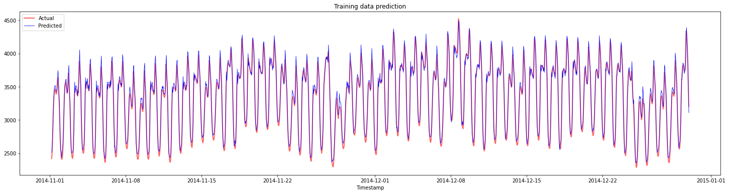
绘制训练数据的预测图:
plt.figure(figsize=(25,6))
plt.plot(train_timestamps, y_train, color = 'red', linewidth=2.0, alpha = 0.6)
plt.plot(train_timestamps, y_train_pred, color = 'blue', linewidth=0.8)
plt.legend(['Actual','Predicted'])
plt.xlabel('Timestamp')
plt.title("Training data prediction")
plt.show()
打印训练数据的MAPE
绘制测试数据的预测图
plt.figure(figsize=(10,3))
plt.plot(test_timestamps, y_test, color = 'red', linewidth=2.0, alpha = 0.6)
plt.plot(test_timestamps, y_test_pred, color = 'blue', linewidth=0.8)
plt.legend(['Actual','Predicted'])
plt.xlabel('Timestamp')
plt.show()
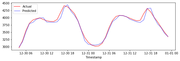
打印测试数据的MAPE
🏆 你在测试数据集上得到了一个非常好的结果!
检查模型在完整数据集上的性能 1
# 提取load值作为numpy数组
data = energy.copy().values

# 缩放
data = scaler.transform(data)

# 根据模型输入要求转换为2D张量
data_timesteps=np.array([[j for j in data[i:i+timesteps]] for i in range(0,len(data)-timesteps+1)])[:,:,0]
print("Tensor shape: ", data_timesteps.shape)

# 从数据中选择输入和输出
X, Y = data_timesteps[:,:timesteps-1],data_timesteps[:,[timesteps-1]]
print("X shape: ", X.shape,"\nY shape: ", Y.shape)
# 进行模型预测
Y_pred = model.predict(X).reshape(-1,1)

# 反向缩放和重塑
Y_pred = scaler.inverse_transform(Y_pred)
Y = scaler.inverse_transform(Y)
plt.figure(figsize=(30,8))
plt.plot(Y, color = 'red', linewidth=2.0, alpha = 0.6)
plt.plot(Y_pred, color = 'blue', linewidth=0.8)
plt.legend(['Actual','Predicted'])
plt.xlabel('Timestamp')
plt.show()
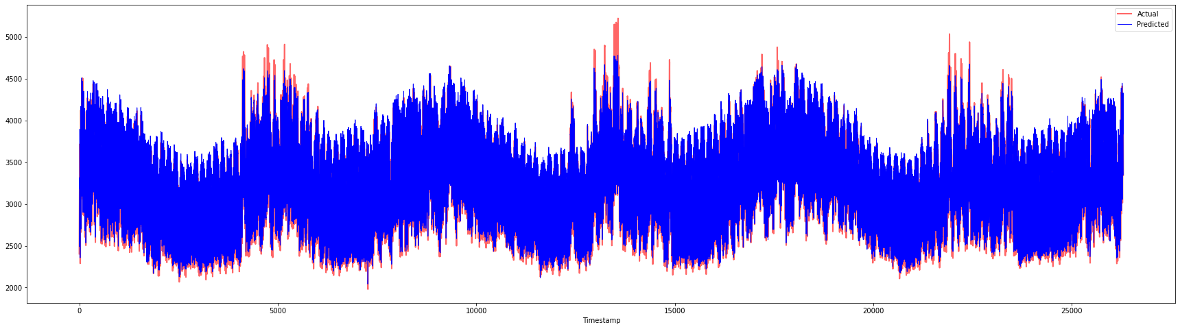
🏆 非常漂亮的图表,显示模型具有良好的准确性。做得好!
🚀挑战
- 尝试在创建模型时调整超参数(gamma, C, epsilon),并在数据上进行评估,看看哪组超参数在测试数据上能得到最好的结果。要了解更多关于这些超参数的信息,可以参考这篇文档。
- 尝试为模型使用不同的核函数,并分析它们在数据集上的性能。可以在这里找到一份有用的文档。
- 尝试使用不同的
timesteps值,让模型回顾不同长度的历史数据来进行预测。
课后测验
复习与自学
本课旨在介绍SVR在时间序列预测中的应用。要了解更多关于SVR的信息,你可以参考这篇博客。这份scikit-learn上的文档对SVMs整体、SVRs以及其他实现细节,如可以使用的不同核函数及其参数,提供了更全面的解释。